Shaker Synchronized Serial Acquisition Template (with NI-DAQmx)
Table of Contents
1 Introduction
This VI project is written as a template that can be followed to develop labview applications for serial hardware where synchronized analog input and output is desired. This document will provide an outline of the basic design of the front panel with its functionality, the block diagram, and a short usage example.
Considerable credit needs to go to the developers of the Impact Testing (DAQmx) sample project which is a part of the Sound and Vibrations toolbox. Much of the front panel as well as block diagram design philosophy (and also code blocks) are from this template.
Please contact me at nidish@iitm.ac.in in case you have questions.
1.1 Prerequisites
For editing and modifying the VI(s) you need to have a LabVIEW license (version>2021) along with the LabVIEW Sound and Vibration Toolkit.
For just running the built applications, a LabVIEW license is not necessary but you need to install
- The LabVIEW Run-Time Engine
- A data plugin for UFF file exports
2 Design of VI
2.1 Front Panel and Features
Figure 1 shows the organization of the VI's front panel. Broadly it is split into 3 palettes: (i) the control palette, (ii) the data palette, and (iii) the display palette.
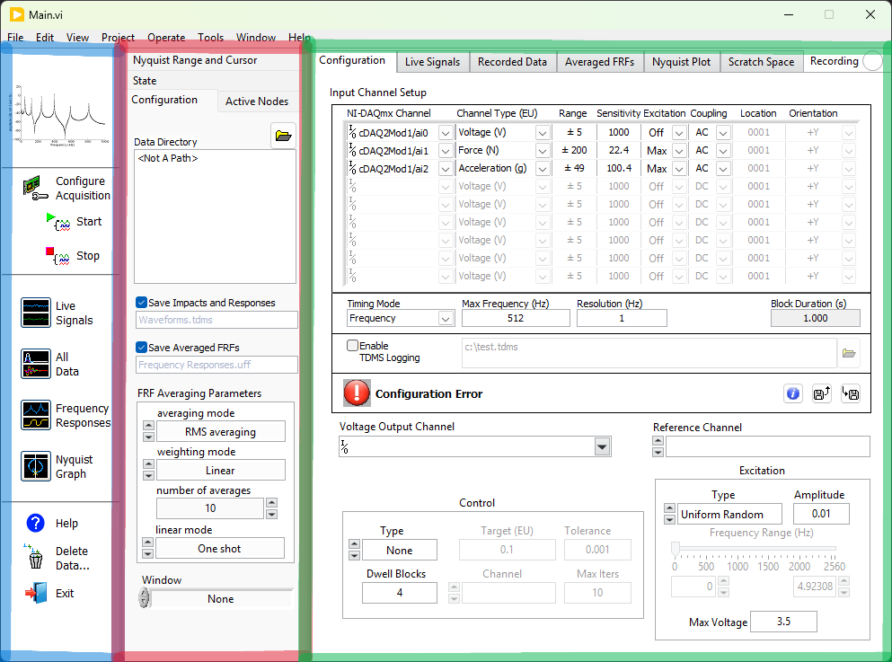
Figure 1: Overview of the front panel showing the control palette (blue), data palette (red), and display palette (green).
2.1.1 Control Palette
The control palette provides buttons for controlling the flow of the program. Specifically we have:
- Configure Aquisition - this will make the Configuration tabs
of the other two palettes active so that the user provide
experimental information.
- The "Start" and "Stop" buttons below this can be used to run and terminate the experiments respectively.
- Live Signals - this will open up the "Active Nodes" and the "Live Signals" tabs in the other two panels respectively.
- All Data - this will open up the "State" and "Recorded Data" tabs in the other two panels respectively.
- Frequency Responses - this will open up the "State"and Äveraged FRFs" tabs respectively.
- Nyquist Graph - this will open up the "Nyquist Range and Cursor" and "Nyquist Plot" tabs.
- The Help button opens up this page.
- The Delete Data… button opens up a prompt asking which data to delete from current acquisition.
- The Exit button exits the VI application .
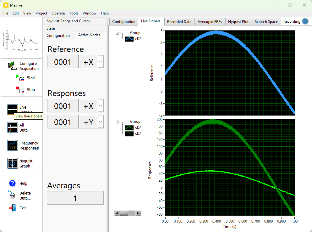
Figure 2: State of the front panel after clicking on "Live Signals"
2.1.2 Data Palette
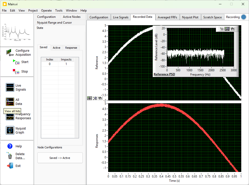
Figure 3: State of the front panel after clicking on "All Data"
The data palette has 5 tabs:
- Configuration: Set the file names to save here. Controls are also provided for FRF averaging and windowing parameters.
- Active Nodes: This lists out the node that is taken as reference along with the nodes that have been taken as responses. It also indicates the number of averages that have been completed for the FRF analysis. (see fig. 2).
- State: This lists out a summary of the data that is current stored. This allows one to choose which of the saved datasets to visualize, etc. (see fig. 3).
- Nyquist Range and Cursor: This lists out parameters helpful for the Nyquist plot visualization (see 4).
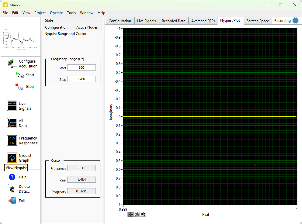
Figure 4: State of the front panel after clicking on "Nyquist Graph"
2.1.3 Display Palette
The display palette has 6 tabs. The last tab, named "Scratch Space", is merely for development purposes and can be used for monitoring the program. Other than this we have,
- Configuration: (see fig. 1) Provide all the
information necessary for conducting the tests.
- The "Reference Channel" is used for the FRF estimates.
- The "Control" cluster sets the parameters for the control.
- If Type is set to None, then each realization of the random excitation is repeated as many times as Dwell Blocks (4 by default) and the response to the last one is saved.
- If Type is set to RMS, then a channel must be selected along
with a target RMS (in its own engineering units). The tolerance
signifies how close we need to come to the target to deem the
responses as converged. Max Iters specifies the maximum
number of iterations to look for convergence (each iteration
involves dwelling before update).
- A secant based update is employed for the "solve".
- The "Excitation" cluser sets the parameters for excitation.
- If _Type is "Uniform Random", then the excitation is chosen by taking voltage values between -Amplitude and +Amplitude .
- If Type is "Gaussian Random", then samples from a Gaussian distribution with zero mean and "Amplitude" standard deviation are provided.
- If Type is "MultiSine Random", then the excitation is a band limited multisine periodic random signal with the band to be selected in the "Frequency Range (Hz)" control below it.
- Live Signals: Merely plots out the reference as well as all the channels as they are running (without requiring convergence, just for visualization).
- Recorded Data: Plots the recorded data in the time domain (different sets can be chosen in Data Palette->Active Nodes) .
- Averaged FRFs: Plots the averaged FRFs along with Coherence and Phase.
- Nyquist Plot: Provides the Nyquist Diagram.
2.2 Structure of the Block Diagram
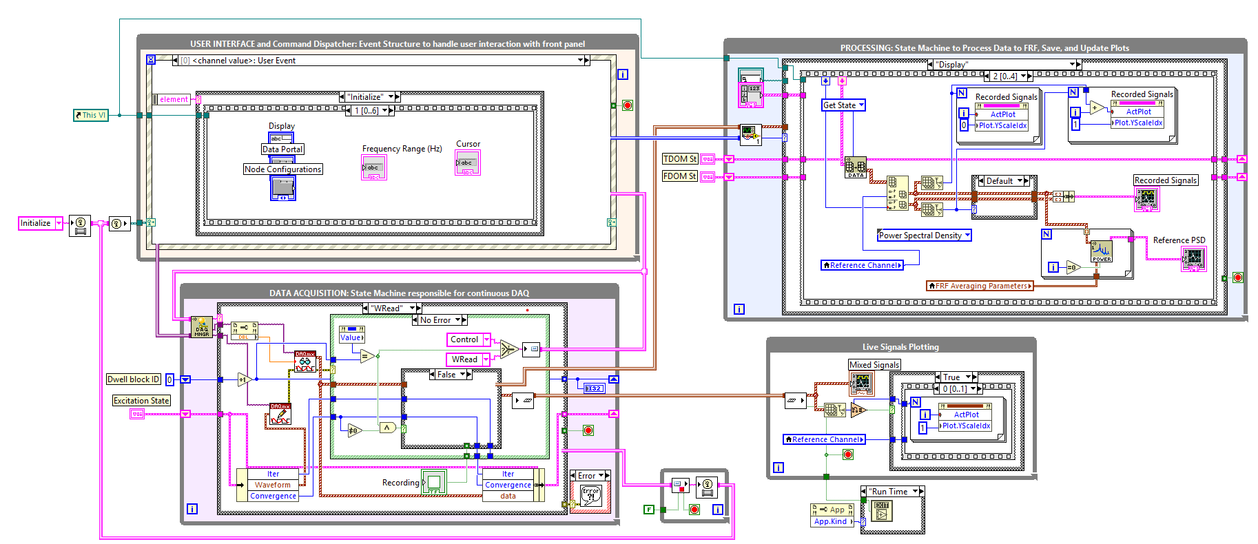
Figure 5: Overview of the block diagram
Figure 5 presents the block diagram for the program. It has 4 main while loops:
- USER INTERFACE: This is what is always waiting for a user event (such as button click, etc.). Based on the input received it sends an appropriate message to one or many of the other while loops running.
- DATA ACQUISITION: As soon as the "Start" button in the data palette is pressed, the data acquisition loop starts running. This starts the tasks and writes/reads the necessary data.
- Live Signals Plotting: DATA ACQUISITION keeps streaming the data as it comes in to this loop. This just plots the data in the "Live Signals" tab.
- PROCESSING: The approved/converged data blocks are sent here. This saves and updates a "Time Domain State" which is capable of managing data from multiple different hits, etc. It also estimates the FRF and does the remaining visualizations.
3 Usage Steps
The steps for general usage are as follows:
- Input channel information. Decide how many tests to do and set
the averaging parameters.
- Do not forget to input unique nodes and directions in the node table.
- Choose the output, setup excitation (Uniform Random at low amplitudes is usually a good starting choice).
- Specify the control parameters if necessary.
- Secant control is used for RMS control. Here a secant update is provided at each iteration, after which the same updated waveform is provided "Dwell Blocks" number of times (for transients to die down, etc.). After convergence, the saving is done.
- Select files for saving if necessary.
- If you desire ALL the data to be logged at all times (irrespective of control, etc.), you may specify the same by choosing the "Enable TDMS Logging" and providing a file name.
- Check everything and hit "Start". This should take you to the live signals and the acquisition would've started.
- Wait for the experiment to complete and export your data.
- You can visualize the FRF and Nyquist for all the sensors by using the GUI interface.
4 Outro
This was made strictly for research purposes and comes with no guarantees of correctness. If you find something wrong, please try to fix it and reach out to me at nidish@iitm.ac.in.
Figure 6 shows me using this setup for testing a clamped beam.
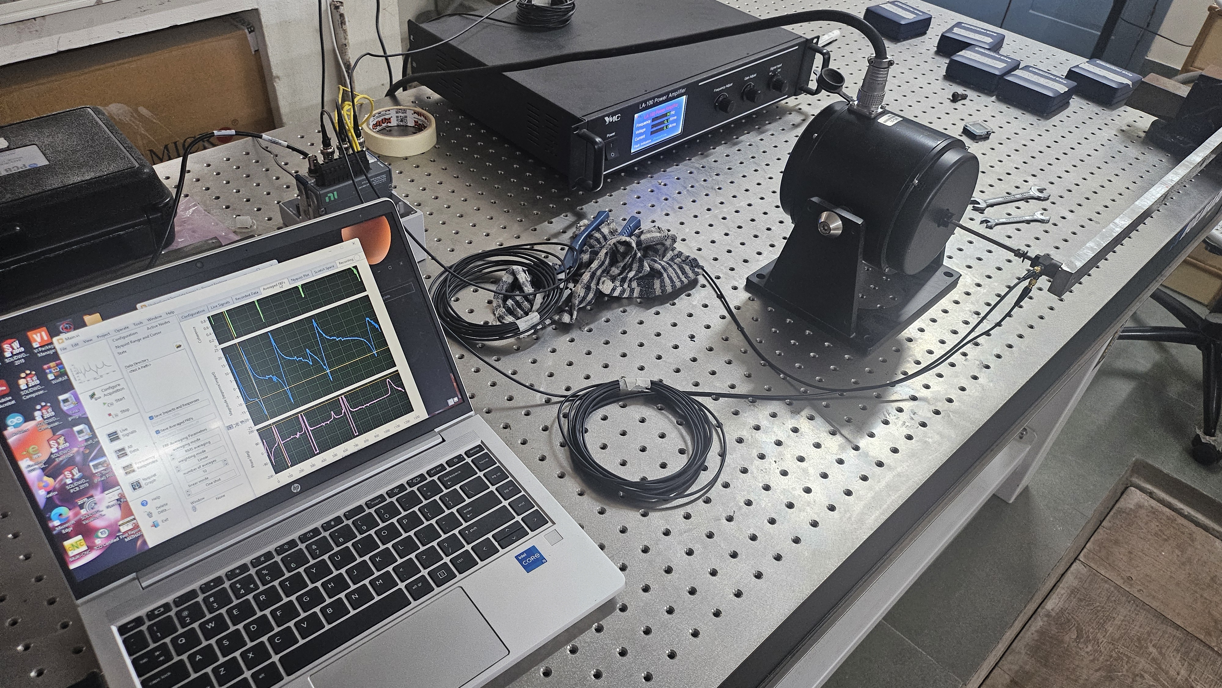
Figure 6: Happy Testing! :-)